Data Assimilation

What is Data Assimilation ?

Data Assimilation is an approach / method for combining high-fidelity observations with low-fidelity model output to improve the latter.

We want to predict the state of the system and its future in the best possible way.

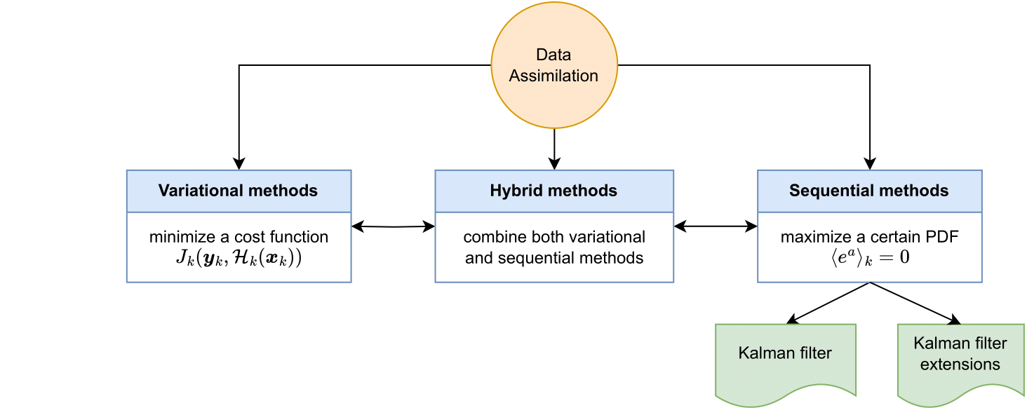
Data assimilation available methods.

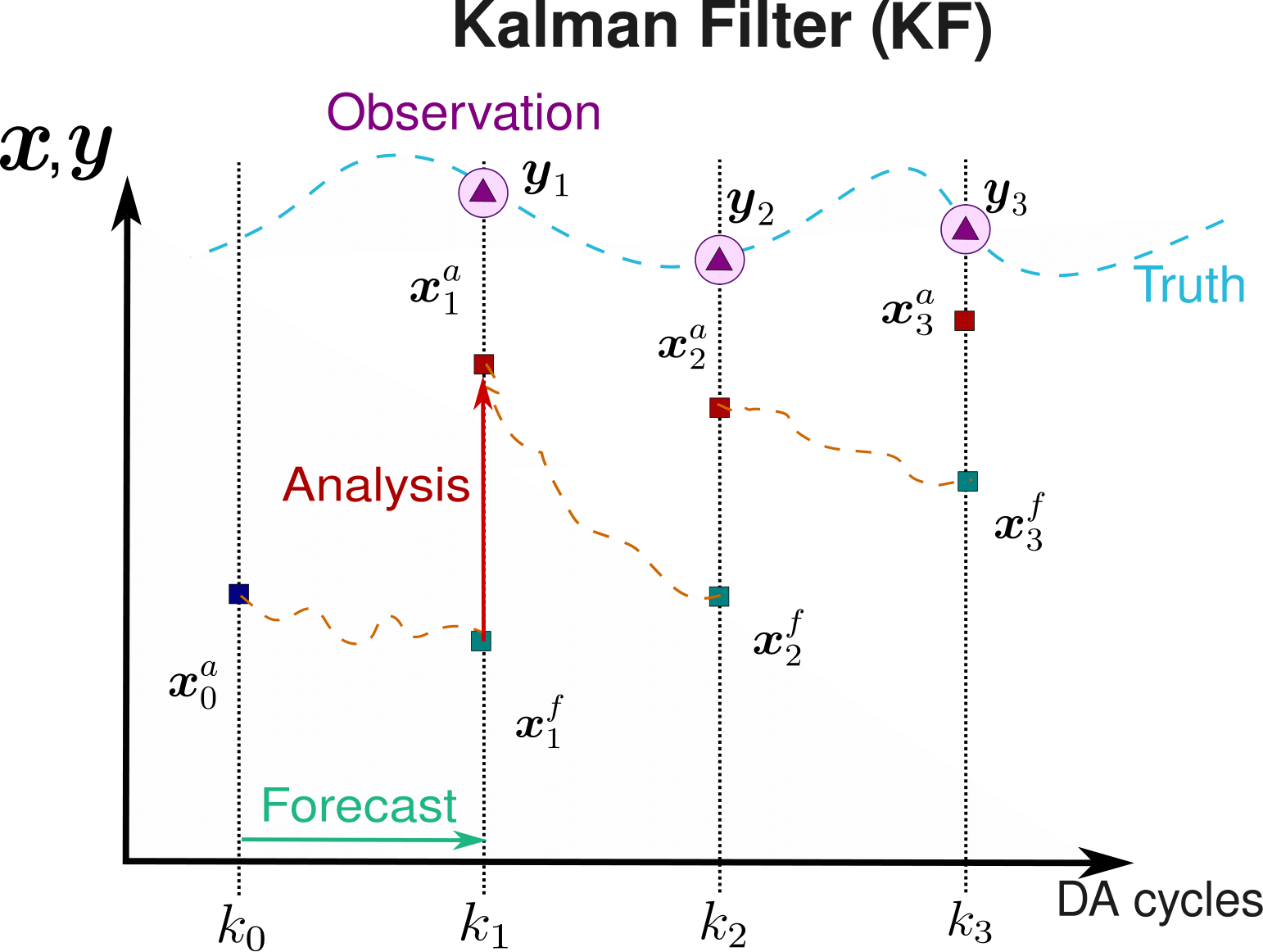
Sequential Data Assimilation : Kalman Filter

Initialization: initial estimate for \(\mathbf{x}^a_0\).

At every \(k\) Data Assimilation cycle,

1. Prediction / Forecast step: the forecast state \(\mathbf{x}_k^f\) is given by the foreward model \(\mathcal{M}_{k-1:k}\) of our system.

2. Correction / analysis step: we perform a correction of the state \(\mathbf{x}_k^a\) based on the forecast state \(\mathbf{x}_k^f\) and some high-fidelity observation \(\mathbf{y}_k\) through the estimation of the so-called Kalman gain matrix \(\mathbf{K}_k\) that minimizes the error covariance matrix of the updated state \(\mathbf{P}_k^a\).

Kalman Filter algorithm scheme.

The inconveniences of the Kalman Filter are:

1. The Kalman Filter - also the Extended Kalman Filter (EKF) - only works for moderate deviations from linearity and Gaussianity:

\[\begin{equation} \mathcal{M}_{k:k-1} \rightarrow \textrm{Navier-Stokes equations (non-linear)} \end{equation}\]

1. High dimensionality of the error covariance matrix \(\mathbf{P}_k\), with a number of degree of freedom equal to \(n_{\textrm{vars}} \times n_{\textrm{cells}}\):

\[\begin{equation} \left[ \mathbf{P}_k \right]_{n_{\textrm{vars}} \times n_{\textrm{cells}}, n_{\textrm{vars}} \times n_{\textrm{cells}}} \end{equation}\]

The possible alternatives to the KF are:

1. Particle filter: cannot yet to be applied to very high dimensional systems (\(m\) = size the ensemble).

2. Ensemble Kalman Filter:

   1. High dimensional systems \(\rightarrow\) we avoid the explicit defintion of \(\mathbf{P}_k\).

   2. Non-linear models \(\rightarrow\) Monte-Carlo realisations.

   3. But underestimation of \(\mathbf{P}_k^a\) \(\rightarrow\) inflation and localisation.

Ensemble Kalman Filter with extended state

The system state \(\mathbf{x}_k\) is as follows:

\[\begin{split}\begin{equation} \begin{bmatrix} \mathbf{u}_k \\ \theta_k \end{bmatrix}_{n_{\textrm{vars}} \times n_{\textrm{cells}}+n_\theta, m} \end{equation}\end{split}\]

where:

• \(\mathbf{u}_k\) is the state matrix (can contain velocities, pressure, temperature…) of the domain at the time instant \(k\).

• \(\theta_k\) are the coefficients from the model we want to infer at the time instant \(k\).

The observation data \(\mathbf{y}_k\) is defined as

\[\begin{equation} \left[ \mathbf{y}_k \right]_{n_{\textrm{obs}},m} \rightarrow \mathcal{N} \left( y_k, \mathbf{R}_k \right) \end{equation}\]

Observation data may be built using:

1. Velocity, pressure, temperature and more… values.

2. Instantaneous global force coefficients \(C_D\), \(C_L\), \(C_f\), …

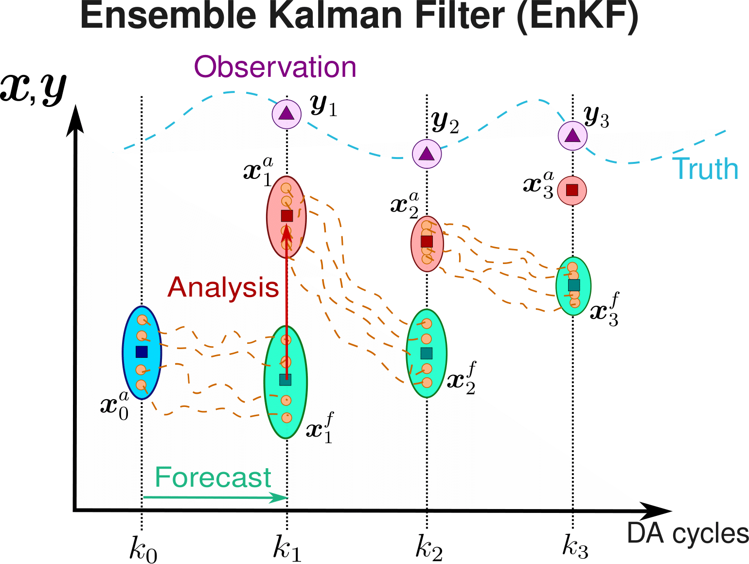
Ensemble Kalman Filter algorithm scheme.

The following matrices are needed to build the EnKF algorithm:

1. Observation covariance matrix \(\mathbf{R}_k\): we assume Gaussian, non-correlated incertainty for the observations (\(\sigma_{i,k}\) is the standard deviation for the variable \(i\) at time instant \(k\)).

\[\begin{equation} \left[ \mathbf{R}_k \right]_{n_{\textrm{obs}}, n_{\textrm{obs}}} = \sigma^2_{i,k} \, \left[ \mathbf{I} \right]_{n_{\textrm{obs}}, n_{\textrm{obs}}} \end{equation}\]

2. Sampling matrix \(\mathcal{H} \left( \mathbf{x}^f_i \right)\): it is the projection the model into the position of the observations.

\[\begin{equation} \left[ \mathcal{H} \left( \mathbf{x}^f_k \right) \right]_{n_{\textrm{obs}},m} \end{equation}\]

3. Anomaly matrices for the system’s state \(\mathbf{x}^f_k\) and sampling \(\mathcal{H} \left( \mathbf{x}^f_i \right) = \mathbf{s}^f_k\) matrices. They measure the deviation of each realisations with respect to the mean.

\[\begin{equation} \mathbf{X} _i =\frac{\mathbf{x}_i - {\overline{\mathbf{x}_i}}}{\sqrt{m-1}} \quad , \quad \mathbf{X} _i =\frac{\mathbf{x=s}_i - {\overline{\mathbf{s}_i}}}{\sqrt{m-1}} \end{equation}\]

\[\begin{equation} \textrm{ with } \quad \left[ \mathbf{X} \right]_{n_{\textrm{vars}} \times n_{\textrm{cells}}+n_\theta, m} \quad , \quad \left[ \mathbf{S} \right]_{n_{\textrm{obs}}, m} \end{equation}\]

4. Kalman Gain matrix:

\[\begin{equation} \mathbf{K} = \mathbf{X} \mathbf{S}^\top \left( \mathbf{S} \mathbf{S}^\top + \mathbf{R} \right)^{-1} \end{equation}\]

\[\begin{equation} \textrm{ with } \quad \left[ \mathbf{K}_k \right]_{n_{\textrm{vars}} \times n_{\textrm{cells}}+n_{\theta},n_{\textrm{obs}}} \end{equation}\]

Multigrid Ensemble Kalman Filter (MGEnKF)

MultiFidelity Ensemble Kalman Filter (MFEnKF)

The MFEnKF is built using 3 sources of information:

1. The principal members, denoted as \(X_i\)

2. The control members, denoted as \(\hat{U}_i\)

3. The ancillary members, denoted as \(U_i\)

Control members \(\hat{U}_i\) are a projection of the principal members \(X_i\) using the projection operator \(\mathbf{\Phi}_r^\star\):

\[\hat{U}_i = \mathbf{\Phi}^*_r \left(X_i \right)\]

The MFEnKF methodology is sketched below, from [popov_multifidelity_2021]:

The Kalman gain \(\tilde{K}_i\) is computed using the 3 ensemble types.

Ensemble means

\[\begin{split}\begin{aligned} \tilde{\mu}_X &= N_X^{-1} E_X 1_{N_X}, \\ \tilde{\mu}_{\hat{U}} &= N_X^{-1} E_{\hat{U}} 1_{N_X}, \\ \tilde{\mu}_U &= N_U^{-1} E_U 1_{N_U}, \\ \tilde{\mu}_{\mathcal{H}(X)} &= N_o^{-1} E_{H(X)} 1_{N_o}, \\ \tilde{\mu}_{H(\hat{U})} &= N_o^{-1} E_{H(\hat{U})} 1_{N_o}, \\ \tilde{\mu}_{H(U)} &= N_o^{-1} E_{H(U)} 1_{N_o}\end{aligned}\end{split}\]

Ensemble anomaly matrices

\[\begin{split}\begin{aligned} A_X &= \left( E_X - \tilde{\mu}_X 1_{N_X}^\top \right) \left( N_X - 1 \right)^{-\frac{1}{2}}, \\ A_{\hat{U}} &= \left( E_{\hat{U}} - \tilde{\mu}_{\hat{U}} 1_{N_X}^\top \right) \left( N_X - 1 \right)^{-\frac{1}{2}}, \\ A_U &= \left( E_U - \tilde{\mu}_U 1_{N_U}^\top \right) \left( N_U - 1 \right)^{-\frac{1}{2}}, \\ A_{H(X)} &= \left( E_{H(X)} - \tilde{\mu}_{H(X)} 1_{N_o}^\top \right) \left( N_X - 1 \right)^{-\frac{1}{2}}, \\ A_{H(\hat{U})} &= \left( E_{H(\hat{U})} - \tilde{\mu}_{H(\hat{U})} 1_{N_o}^\top \right) \left( N_X - 1 \right)^{-\frac{1}{2}}, \\ A_{H(U)} &= \left( E_{H(U)} - \tilde{\mu}_{H(U)} 1_{N_o}^\top \right) \left( N_U - 1 \right)^{-\frac{1}{2}}\end{aligned}\end{split}\]

Ensemble covariances

\[\begin{split}\begin{aligned} \tilde{\Sigma}_{X,H(X)} &= A_X A_{H(X)}^\top \\ \tilde{\Sigma}_{\hat{U},H(\Phi_r \hat{U})} &= A_{\hat{U}} A_{H(\Phi_r \hat{U})}^\top \\ \tilde{\Sigma}_{X,H(\Phi_r \hat{U})} &= A_X A_{H(\Phi_r \hat{U})}^\top \\ \tilde{\Sigma}_{\hat{U},H(X)} &= A_{\hat{U}} A_{H(X)}^\top \\ \tilde{\Sigma}_{U,H(\Phi_r U)} &= A_U A_{H(\Phi_r U)}^\top \\ \tilde{\Sigma}_{H(X),H(X)} &= A_{H(X)} A_{H(X)}^\top \\ \tilde{\Sigma}_{H(\Phi_r \hat{U}),H(\Phi_r \hat{U})} &= A_{H(\Phi_r \hat{U})} A_{H(\Phi_r \hat{U})}^\top \\ \tilde{\Sigma}_{H(X),H(\Phi_r \hat{U})} &= A_{H(X)} A_{H(\Phi_r \hat{U})}^\top \\ \tilde{\Sigma}_{H(\Phi_r \hat{U}),H(X)} &= A_{H(\Phi_r \hat{U})} A_{H(X)}^\top \\ \tilde{\Sigma}_{H(\Phi_r U),H(\Phi_r U)} &= A_{H(\Phi_r U)} A_{H(\Phi_r U)}^\top \end{aligned}\end{split}\]

Kalman gain intermediate covariances

\[\begin{split}\begin{aligned} \tilde{\Sigma}_{Z, H(Z)} &= \tilde{\Sigma}_{X,H(X)} + \frac{1}{4} \Phi_r \tilde{\Sigma}_{\hat{U},H(\Phi_r \hat{U})} - \frac{1}{2} \tilde{\Sigma}_{X,H(\Phi_r \hat{U})} - \frac{1}{2} \Phi_r \tilde{\Sigma}_{\hat{U},H(X)} + \frac{1}{4} \Phi_r \tilde{\Sigma}_{U,H(\Phi_r U)} \\ \tilde{\Sigma}_{H(Z), H(Z)} &= \tilde{\Sigma}_{H(X),H(X)} + \frac{1}{4} \tilde{\Sigma}_{H(\Phi_r \hat{U}),H(\Phi_r \hat{U})} - \frac{1}{2} \tilde{\Sigma}_{H(X),H(\Phi_r \hat{U})} - \frac{1}{2} \tilde{\Sigma}_{H(\Phi_r \hat{U}),H(X)} + \frac{1}{4} \tilde{\Sigma}_{H(\Phi_r U),H(\Phi_r U)}\end{aligned}\end{split}\]

Computing Kalman Gain

\[\tilde{K} = \tilde{\Sigma}_{Z, H(Z)} \left( \tilde{\Sigma}_{H(Z), H(Z)} + \tilde{\Sigma}_{\eta,\eta} \right)^{-1}\]

Update and total variate

Each variable can be updated:

\[\begin{split}\begin{aligned} X^a &= X^f + \tilde{K} \left( y - H(X) \right) \\ \hat{U}^a &= \hat{U}^f + \Phi_r^* \tilde{K} \left( y - H(\hat{U}) \right) \\ U^a &= U^f + \Phi_r^* \tilde{K} \left( y - H(U) \right) \end{aligned}\end{split}\]

The total variate Z represents the combined prior and posterior knowledge through the linear control variate technique:

\[\begin{split}\begin{aligned} Z^f &= X^f - S \left( \hat{U}^f - \overline{U^f} \right) \\ Z^a &= X^a - S \left( \hat{U}^a - \overline{U^a} \right)\end{aligned}\end{split}\]

where S = |Phi_r| / 2